Surface source Example

Estimate NCRFs for standard and oddball tones.

For this tutorial, we use the auditory Brainstorm tutorial dataset [Tadel et al., 2011] that is available as a part of the Brainstorm software.

Note

Downloading the dataset requires answering an interactive prompt (see mne.datasets.brainstorm.bst_auditory.data_path()).

# Authors: Proloy Das <proloy@umd.edu>
#          Christian Brodbeck <brodbecc@mcmaster.ca>
#
# sphinx_gallery_thumbnail_number = 3

import numpy as np
import pandas as pd
import eelbrain
import mne
from ncrf import fit_ncrf

Preprocessing

Preprocess MEG Data: low pass filtering, power line attenuation, downsampling, etc. We broadly follow this mne-python tutorial.

data_path = mne.datasets.brainstorm.bst_auditory.data_path()
raw_fname = data_path / 'MEG' / 'bst_auditory' / 'S01_AEF_20131218_01.ds'
raw = mne.io.read_raw_ctf(raw_fname, preload=False)
n_times_run1 = raw.n_times

# We mark a set of bad channels that seem noisier than others.
raw.info['bads'] = ['MLO52-4408', 'MRT51-4408', 'MLO42-4408', 'MLO43-4408']

annotations_df = pd.DataFrame()
offset = n_times_run1
for idx in [1]:
    csv_fname = data_path / 'MEG' / 'bst_auditory' / f'events_bad_0{idx}.csv'
    df = pd.read_csv(csv_fname, header=None, names=['onset', 'duration', 'id', 'label'])
    print('Events from run {0}:'.format(idx))
    print(df)

    df['onset'] += offset * (idx - 1)
    annotations_df = pd.concat([annotations_df, df], axis=0)

# Conversion from samples to times:
onsets = annotations_df['onset'].values / raw.info['sfreq']
durations = annotations_df['duration'].values / raw.info['sfreq']
descriptions = annotations_df['label'].values

annotations = mne.Annotations(onsets, durations, descriptions)
raw.set_annotations(annotations)
del onsets, durations, descriptions


# events are the presentation times of the audio stimuli: UPPT001
event_fname = data_path / 'MEG' / 'bst_auditory' / 'S01_AEF_20131218_01-eve.fif'
events = mne.find_events(raw, stim_channel='UPPT001')
# The event timing is adjusted by comparing the trigger times on detected sound onsets on channel UADC001-4408.
sound_data = raw[raw.ch_names.index('UADC001-4408')][0][0]
onsets = np.where(np.abs(sound_data) > 2. * np.std(sound_data))[0]
min_diff = int(0.5 * raw.info['sfreq'])
diffs = np.concatenate([[min_diff + 1], np.diff(onsets)])
onsets = onsets[diffs > min_diff]
assert len(onsets) == len(events)
diffs = 1000. * (events[:, 0] - onsets) / raw.info['sfreq']
print('Trigger delay removed (μ ± σ): %0.1f ± %0.1f ms'
      % (np.mean(diffs), np.std(diffs)))

# events times are rescaled according to new sampling freq, 100 Hz
events[:, 0] = np.int64(onsets * 100 / raw.info['sfreq'])
mne.write_events(event_fname, events, overwrite=True)

del sound_data, diffs

## set EOG channel
raw.set_eeg_reference('average', projection=True)
# raw_AEF.plot_psd(tmax=60., average=False)
raw.load_data()
raw.notch_filter(np.arange(60, 181, 60), fir_design='firwin')

# band pass filtering 1-8 Hz
raw.filter(1.0, 8.0, fir_design='firwin')

# resample to 100 Hz
raw.resample(100, npad="auto")

### LOAD RELEVANT VARIABLES AS eelbrain.NDVar
# load as epochs for plot only
ds = eelbrain.load.fiff.events(raw=raw, proj=True, stim_channel='UPPT001', events=event_fname)
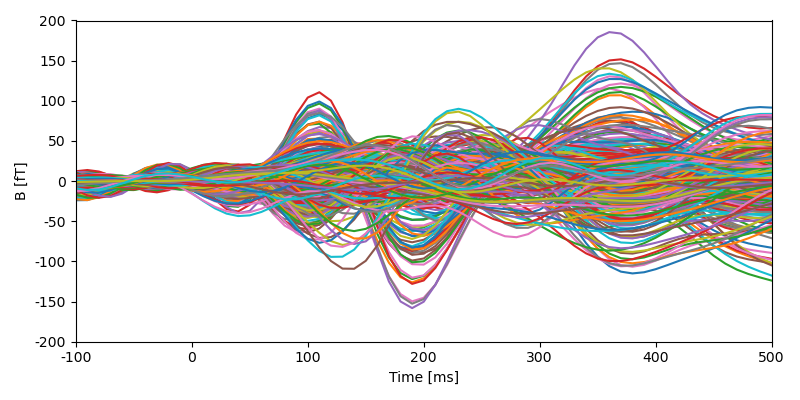
epochs = eelbrain.load.fiff.epochs(ds, tmin=-0.1, tmax=0.5, baseline=(None, 0))
eelbrain.plot.Butterfly(epochs)

# pick MEG channels
picks = mne.pick_types(raw.info, meg=True, eeg=False, stim=False, eog=False,
                       ref_meg=False, exclude='bads')

# Read as a single chunk of data
y, t = raw.get_data(picks, return_times=True)
sensor_dim = eelbrain.load.fiff.sensor_dim(raw.info, picks=picks)
time = eelbrain.UTS.from_int(0, t.size - 1, raw.info['sfreq'])
meg = eelbrain.NDVar(y, dims=(sensor_dim, time))
print(meg)

Events from run 1:
     onset  duration  id label
0     7625      2776   1   BAD
1   142459       892   1   BAD
2   216954       460   1   BAD
3   345135      5816   1   BAD
4   357687      1053   1   BAD
5   409101      3736   1   BAD
6   461110       179   1   BAD
7   479866       426   1   BAD
8   764914     11500   1   BAD
9   798174      6589   1   BAD
10  846880      5383   1   BAD
11  858863      5136   1   BAD
Trigger delay removed (μ ± σ): -13.9 ± 0.3 ms
/home/runner/mne_data/MNE-brainstorm-data/bst_auditory/MEG/bst_auditory/S01_AEF_20131218_01.ds/S01_AEF_20131218_01.meg4: MNE generated only 233 Epochs for 240 events. The raw file might end before the end of the last epoch.
<NDVar: 270 sensor, 36000 time>

Continuous stimulus variable construction

After loading and processing the raw data, we will construct the predictor variable for this particular experiment (by putting an impulse at every event time-point). Note that, the predictor variable and meg response should be of same length.

In case of repetitive trials (where you will have a eelbrain.Case dimension), supply one predictor variable for each trial. Different predictor variables for a single trial can be nested (see ncrf.fit_ncrf()).

In this example, we use two different predictor variables for a single trial

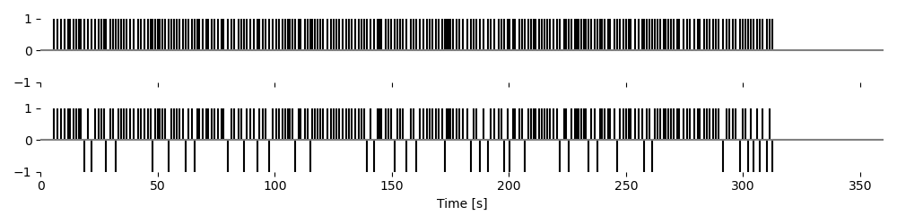
# For the common response, we put impulses at the presentation times of both the audio stimuli (i.e., all beeps).
stim1 = np.zeros(len(time))
stim1[events[:, 0]] = 1.

# To distinguish between standard and deviant beeps, we assign 1 and -1 impulses respectively.
stim2 = stim1.copy()
stim2[events[np.where(events[:, 2] == 2), 0]] = -1.
stim1 = eelbrain.NDVar(stim1, time)
stim2 = eelbrain.NDVar(stim2, time)

# Visualize the stimulus
# p = eelbrain.plot.LineStack(eelbrain.combine([stim1, stim2]), w=10, h=2.5, legend=False)
p = eelbrain.plot.UTS([stim1, stim2], color='black', stem=True, frame='none', w=10, h=2.5, legend=False)

Noise covariance estimation

Here we estimate the noise covariance from empty room data. Instead, you can also use pre-stimulus recordings to compute noise covariance.

noise_path = data_path / 'MEG' / 'bst_auditory' / 'S01_Noise_20131218_01.ds'
raw_empty_room = mne.io.read_raw_ctf(noise_path, preload=True)

# Apply the same pre-processing steps to empty room data
raw_empty_room.notch_filter(np.arange(60, 181, 60), fir_design='firwin')

raw_empty_room.filter(1.0, 8.0, fir_design='firwin')

raw_empty_room.resample(100, npad="auto")

# Compute the noise covariance matrix
noise_cov = mne.compute_raw_covariance(raw_empty_room, tmin=0, tmax=None, method='shrunk', rank=None)

Forward model (aka lead-field matrix)

Now is the time for forward modeling. ‘ico-4’ should be sufficient resolution if working with surface source space. You can choose to work with free or constrained lead fields. :func`ncrf.fit_ncrf` will choose the appropriate regularizer by looking at the provided lead-field matrix.

# The paths to FreeSurfer reconstructions
subjects_dir = data_path / 'subjects'
subject = 'bst_auditory'

# mne.viz.plot_bem(subject=subject, subjects_dir=subjects_dir,
#                  brain_surfaces='white', orientation='coronal')

# The transformation file obtained by coregistration
trans = data_path / 'MEG' / 'bst_auditory' / 'bst_auditory-trans.fif'

# Here we look at the head only.
# mne.viz.plot_alignment(raw.info, trans, subject=subject, dig=True,
#                        meg=['helmet', 'sensors'], subjects_dir=subjects_dir,
#                        surfaces='head')

srcfile = subjects_dir / 'bst_auditory' / 'bem' / 'bst_auditory-ico-4-src.fif'
if srcfile.is_file():
    src = mne.read_source_spaces(srcfile)
else:
    src = mne.setup_source_space(subject, spacing='ico4',
                                 subjects_dir=subjects_dir, add_dist=False)
    mne.add_source_space_distances(src)
    mne.write_source_spaces(srcfile, src, overwrite=True)  # needed for smoothing
src

<SourceSpaces: [<surface (lh), n_vertices=163080, n_used=2562>, <surface (rh), n_vertices=163816, n_used=2562>] MRI (surface RAS) coords, subject 'bst_auditory', ~34.5 MiB>

Compute the forward solution:

fwdfile = subjects_dir / 'bst_auditory' / 'bem' / 'bst_auditory-ico-4-fwd.fif'
if fwdfile.is_file():
    fwd = mne.read_forward_solution(fwdfile)
else:
    conductivity = (0.3,)  # for single layer
    # conductivity = (0.3, 0.006, 0.3)  # for three layers
    model = mne.make_bem_model(subject=subject, ico=4,
                               conductivity=conductivity,
                               subjects_dir=subjects_dir)
    bem = mne.make_bem_solution(model)

    fwd = mne.make_forward_solution(raw.info, trans=trans, src=src, bem=bem,
                                    meg=True, eeg=False, mindist=5.0, n_jobs=2)
    mne.write_forward_solution(fwdfile, fwd)

fwd

[Parallel(n_jobs=2)]: Using backend LokyBackend with 2 concurrent workers.
[Parallel(n_jobs=2)]: Done   2 out of   2 | elapsed:    0.4s finished
[Parallel(n_jobs=2)]: Using backend LokyBackend with 2 concurrent workers.
[Parallel(n_jobs=2)]: Done   2 out of   2 | elapsed:    0.5s finished
[Parallel(n_jobs=2)]: Using backend LokyBackend with 2 concurrent workers.
[Parallel(n_jobs=2)]: Done   2 out of   2 | elapsed:    0.5s finished
[Parallel(n_jobs=2)]: Using backend LokyBackend with 2 concurrent workers.
[Parallel(n_jobs=2)]: Done   2 out of   2 | elapsed:    0.5s finished
[Parallel(n_jobs=2)]: Using backend LokyBackend with 2 concurrent workers.
[Parallel(n_jobs=2)]: Done   2 out of   2 | elapsed:    0.3s finished

	Forward
	Magnetometers	270 and 4 bad
	Source space	Surface with 5107 vertices
	Source orientation	Free

Extract the fixed orientation lead field matrix:

fwd_fixed = mne.convert_forward_solution(
    fwd, surf_ori=True, force_fixed=True, use_cps=True)

# leadfield matrix
lf = eelbrain.load.fiff.forward_operator(fwd_fixed, src='ico-4', subjects_dir=subjects_dir)

NCRF estimation

Now that we have all the required data to estimate NCRFs.

Note

This example uses simplified settings to speed up estimation:

1) For this example, we use a fixed regularization parameter (mu). For a real experiment, the optimal mu would be determined by cross-validation (set mu='auto', which is the default). The optimal mu will then be stored in model.mu (this is how the mu used here was determined).

2) The example forces the estimation to stop after fewer iterations than is recommended (n_iter). For stable models, we recommend to use the default setting (n_iter=10).

# To speed up the example, we cache the NCRF:
ncrf_file = data_path / 'MEG' / 'bst_auditory' / 'oddball_ncrf.pickle'
if ncrf_file.exists():
    model = eelbrain.load.unpickle(ncrf_file)
else:
    model = fit_ncrf(
        meg, [stim1, stim2], lf, noise_cov, tstart=0, tstop=0.5,
        mu=0.0001756774187547859, n_iter=5,
    )
    eelbrain.save.pickle(model, ncrf_file)

The learned kernel/filter (the NCRF) can be accessed as an attribute of the model. NCRFs are stored as eelbrain.NDVar. Here, the two NCRFs correspond to the two different predictor variables:

model.h

[<NDVar: 5107 source, 51 time>, <NDVar: 5107 source, 51 time>]

Visualization

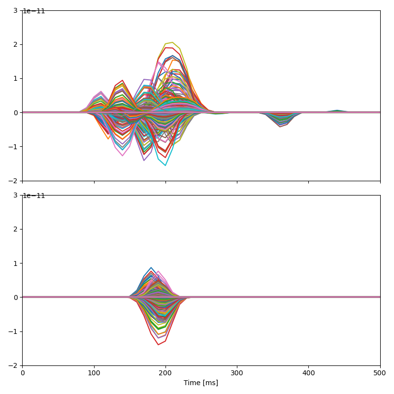
A butterfly plot shows weights in all sources over time. This is good for forming a quick impression of important time lags, or peaks in the response:

Note

Since the estimates are sparse over cortical locations, smoothing the NCRFs over sources to make the visualization more intuitive.

hs = [h.smooth('source', 0.01, 'gaussian') for h in model.h]
p = eelbrain.plot.Butterfly(hs)

The following code for plotting the anatomical localization is commented because the Mayavi based plots do not work reliably in the automatic documentation. Uncomment it to create anatomical plots.

A single time point can be visualized with the PySurfer (surfer) based eelbrain.plot.brain.brain():

# brain = eelbrain.plot.brain.brain(h[0].sub(time=0.140), vmax=2e-11, surf='pial')

An eelbrain.plot.brain.SequencePlotter can be used to plot a sequence of brain images, for example in a jupyter notebook:

# h_binned = h0.bin(0.1, 0.1, 0.4, 'extrema')
# sp = eelbrain.plot.brain.SequencePlotter()
# sp.set_brain_args(surf='inflated')
# sp.add_ndvar(h_binned)
# p = sp.plot_table(view='lateral')

In an interactive iPython session, we can also use interactive time-linked plots with eelbrain.plot.brain.butterfly():

# brain, butterfly = eelbrain.plot.brain.butterfly(h0)

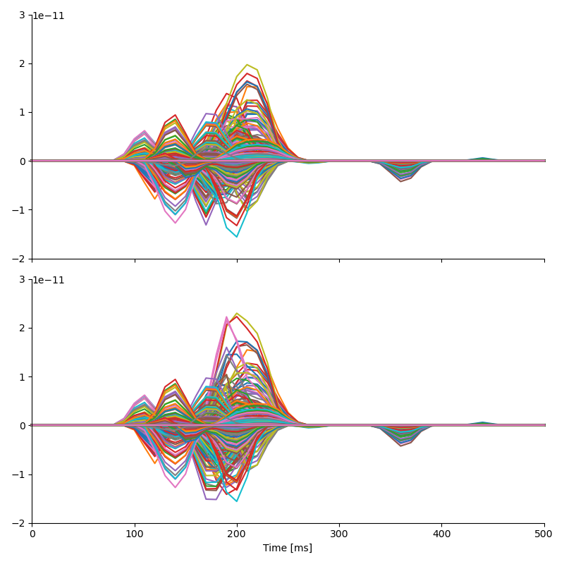
Finally, we can reconstruct the response to frequent and infrequent stimuli as \([Common - Contrast]\) amd \([Common + Contrast]\) respectively.

h_recon = (hs[0] - hs[1], hs[0] + hs[1])
p = eelbrain.plot.Butterfly(h_recon, frame=None)